The concept of a universal calculator, which originated in Britain in the 19th century with Charles Babbage and was developed by Alan M. Turing in the early 20th century, lies at the heart of the first computer’s creation. The development of advanced technology, especially in electronics, paved the way for the creation of the world’s first real computer, the ENIAC, in 1946.
Who invented the first computer?
Using Blaise Pascal’s work as a starting point, Charles Babbage developed the concept of programming.
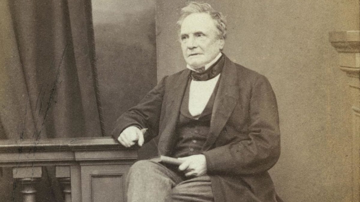
Charles Babbage, an English mathematician, developed the ideas for the first programmed calculating machine between 1834 and 1837. Using Blaise Pascal‘s work as a starting point, this visionary innovator developed the concept of programming using punch cards, which was already in use in the automated creation of music (the Barrel Organ), among other things.
This was the first step toward the development of modern computers. Regrettably, he was unable to realize his vision; the primitive state of technology at the time ensured that his “difference engine” was never produced.
After waiting almost a century, another English mathematician by the name of Alan Turing made a monumental breakthrough in the development of computer technology. In 1936, he wrote, “On computable numbers, with an application to the Entscheidungsproblem” which paved the way for the development of “Turing machines” that unified computation, programming, and computation languages.
Programmable calculators
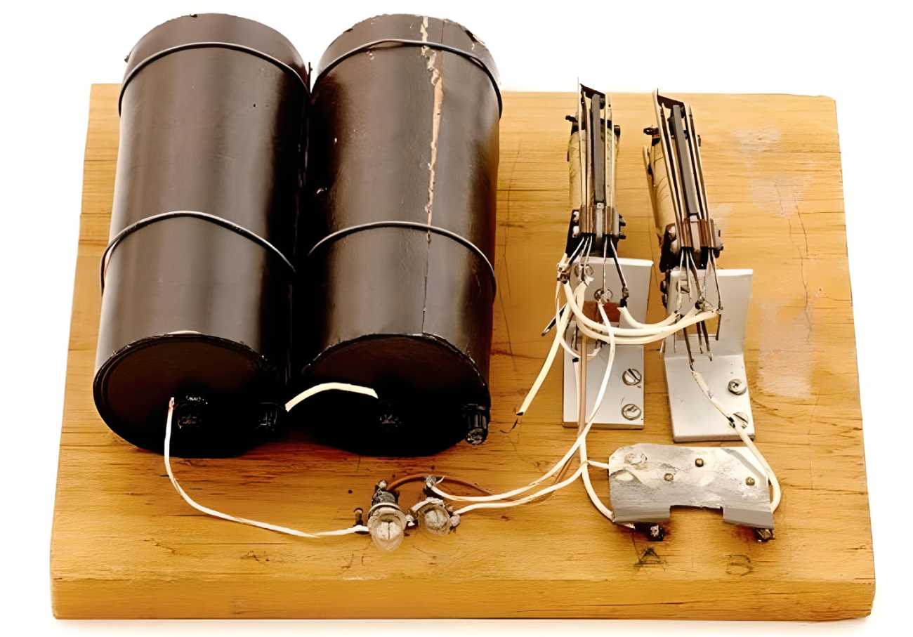
The Model K, 1937.
Major advancements were achieved during World War II, which owes a great deal to the contemporary age of computers. That’s why we ditched making mechanical parts and transitioned to digital computation and electronic circuits, including vacuum tubes, capacitors, and relays. This period saw the creation of the very first generation of computers.
Many programmable calculators appeared between 1937 and 1944:
The “Model K“, developed in a kitchen, 1937.
The “Z-series” computer, 1936.
The Atanasoff-Berry computer, or ABC for short, 1942.
The Complex Number Calculator (CNC), 1939.
The Harvard Mark I computer, 1944.
The “Bombe” vs. “Enigma”
Enigma, late 1930s.
The United Kingdom put forth a significant effort at Bletchley Park during World War II in order to crack the German military’s encrypted communications. Bombes, machines developed by the Polish secret agency and perfected by the British, were used to crack the primary German encryption system, Enigma.
In 1936, Alan Mathison Turing (1912–1954) published “On computable numbers, with an application to the Entscheidungsproblem,” which paved the ground for the development of the programmable computer. He explained his own idea of the computer, which he called “Turing,” the first universal programmable computer, and, by extension, he created the ideas of “program” and “programming.”
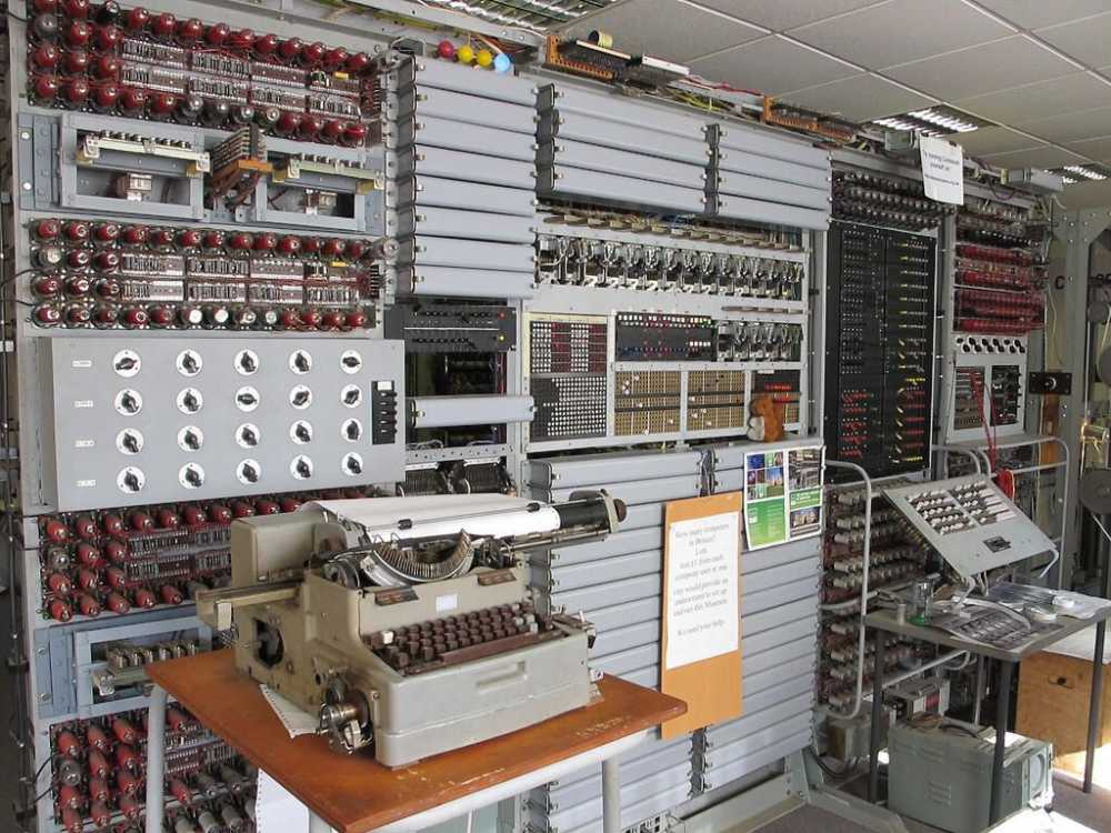
The replica of the first-ever electronic computer in history, the Colossus, 1943. (The National Museum of Computing)
Encryption keys, or ciphers, were discovered using these devices. The Germans developed yet another family of ciphers that were radically different from Enigma; the British dubbed them FISH. Professor Max Newman devised the Colossus, often known as the “Turing bombe,” to crack these systems. It was developed by engineer Tommy Flowers in 1943. The Colossus was later disassembled and buried due to its strategic value.
Colossus was not programmable as it was pre-programmed for a certain task. ENIAC, on the other hand, could be reprogrammed, albeit doing so could take many days. In this sense, ENIAC was the first programmable computer in history.
From ENIAC to modern computer
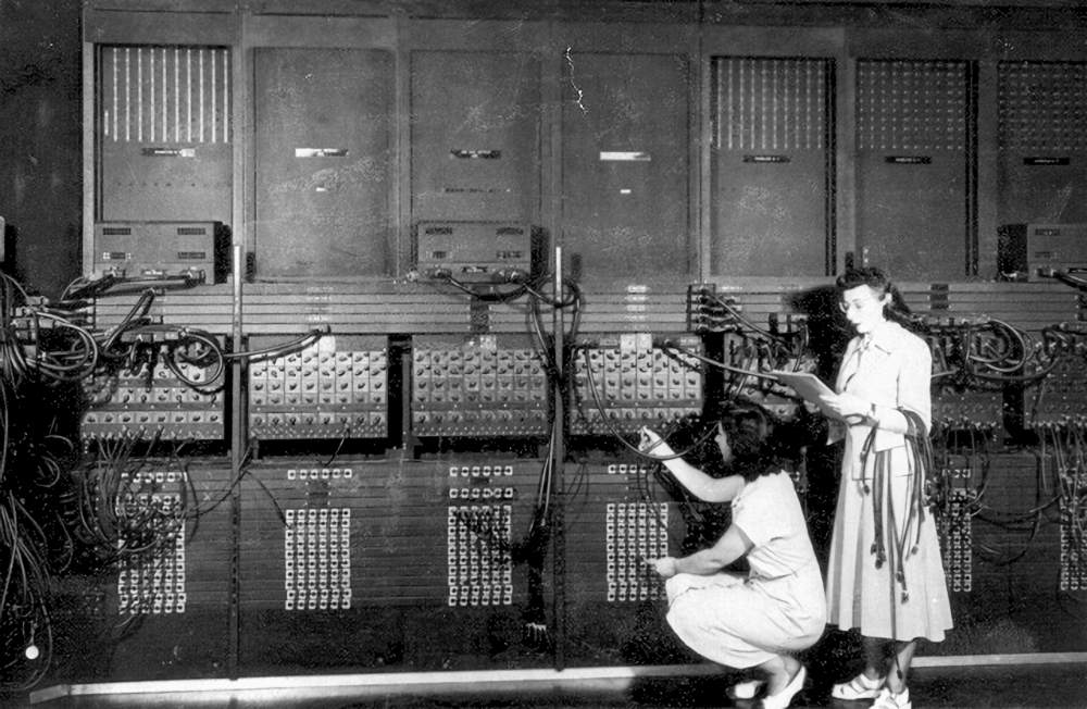
ENIAC, 1945.
The first completely electronic and programmable modern computer to be Turing-complete did not exist until 1946. This was with the ENIAC (Electronic Numerical Integrator and Computer) constructed by Presper Eckert and John William Mauchly.
In 1948, von Neumann architecture computers began appearing. These computers were distinct from their predecessors in that the programs were kept in the same memory as the data. This design allowed the programs to be manipulated just like data. It was pioneered in 1948 by the University of Manchester’s Small-Scale Experimental Machine (SSEM).
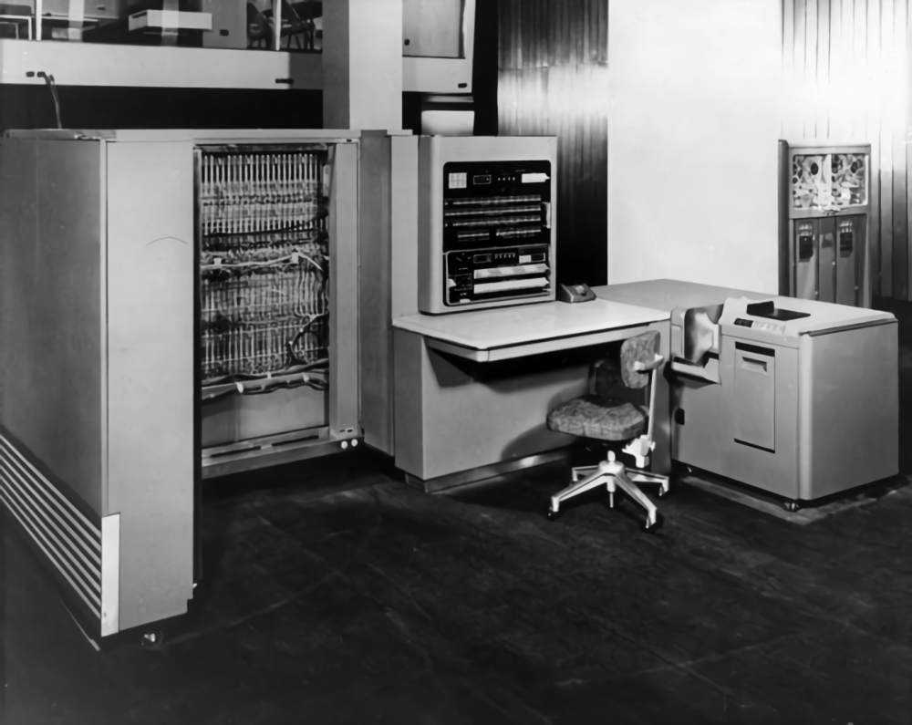
IBM 701 Electronic Data Processing System.
Afterward, IBM released its 701 models in 1952, and subsequent years saw the introduction of the so-called second-generation (1956), third-generation (1963), and fourth-generation (1971) computers, each of which saw the development of the microprocessor and continued the relentless pursuit of miniaturization and computing power.
The innovation of microprocessors, the newest incarnation of which is artificial intelligence, has made desktop computers, laptops, and several high-tech variants (graphics cards, cellphones, touch tablets, etc.) commonplace in our lives today.
The invention of the transistor in December 1947 marked the beginning of a new age in electronics, one in which computers, mobile phones, the Internet, and almost all other electronic devices would not exist without transistors. This semiconductor component has had as much of an impact on technology, society, and daily life as the invention of the wheel or electricity. Let’s have a look at the invention and history of the transistor.
Transistors, in the form of integrated circuits and microchips, can be found in almost every modern electronic device. They are responsible for producing the ones and zeros that are the basis of all digital devices. Simultaneously, they serve as amplifiers, oscillators, and in numerous other fundamental roles in contemporary electronic devices. There were some radical innovations and some detours in the early stages of the development of transistors.
From the vacuum tube to the transistor
The transistor is a really revolutionary development, on par with the wheel and the discovery of fire. It has had maybe the greatest impact on our daily lives and our whole society. Without it, we wouldn’t have desktop computers, laptops, mobile phones, the Internet, or anything else that relies on a microprocessor. Calculator-powered computers would still take up a whole room.
A combination of a switch, rectifier, and amplifier
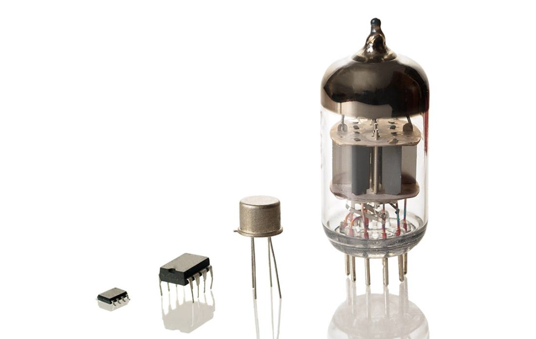
Numerous individual circuits are the foundation of electronics. Today’s microchips (left) use transistors (middle) as switches, while earlier designs used bulky vacuum tubes (right). (Credit: Vlabo/Getty Images)
Most electronic parts and gadgets rely on electrical circuits, which determine whether or not a current flows and under what circumstances. But to do this, you’ll need switches that can be operated by electricity. The flow of a considerably greater current is controlled by a much smaller control current. A computer’s ability to perform digital computing tasks is based on the combination of these switches, or “logic gates,” into circuits. However, this can only be achieved if the electrical switches are very responsive and can be regulated accurately.
In addition, many technological applications need the amplification and modification of electrical signals, such as the production of radar or radio signals, the use of loudspeakers, microphones, and monitors, and the transformation of alternating current (AC) to direct current (DC). Again, the goal is to control the resultant electrical current flow in the most efficient and cost-effective method.
When vacuum tubes were first used
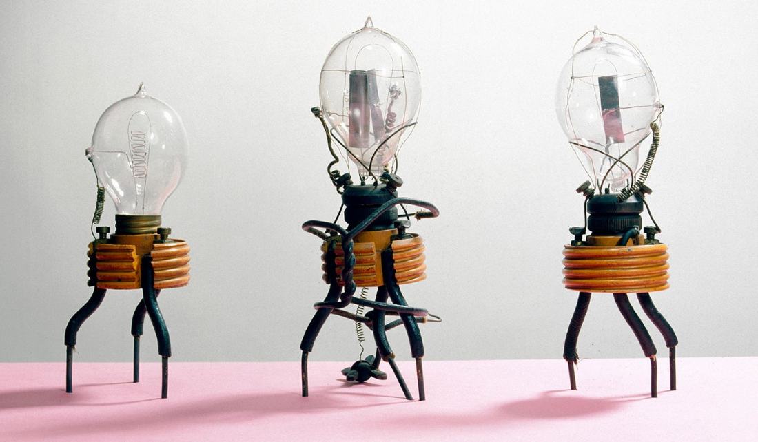
Fleming’s oscillation valve. For use in early radio receivers for electromagnetic wireless telegraphy, English scientist John Ambrose Fleming designed a thermionic valve or vacuum tube in 1904 that he termed the Fleming oscillation valve. (Credit: SSPL/Getty Images)
Mechanical switches in the form of relays were employed for these purposes before the invention of the transistor, but they switched between states slowly. Alternatively, vacuum tubes, which were first developed in 1904, were put into service. They are so-called triodes and are constructed out of an airtight glass, steel, or ceramic tube with three electrodes. With the third electrode in place, the electric field created between the anode and cathode can be used to control the amount of current flowing between the two.
However, vacuum tubes have a number of drawbacks, including their bulk, fragility, and high power requirements for regulation. Cabinets full of vacuum tubes were utilized for the circuits in the early computers, which meant they took up whole rooms. The British employed a machine called Colossus to decipher German signals during WWII. Meanwhile, the Americans were hard at work on ENIAC, the first general-purpose computer. Similarly, the vacuum tubes within the popular tube radios of the day made the receivers seem more like pieces of furniture than portable listening devices.
Another drawback is that the switching speed of tubes is restricted. This is despite the fact that they switch significantly quicker than mechanical relays. The need for rectifiers and amplifiers that could switch in the gigahertz range arose as a pressing issue, particularly during World War II, when the military’s radar systems were upgraded to greater power.
The discovery of semiconductors
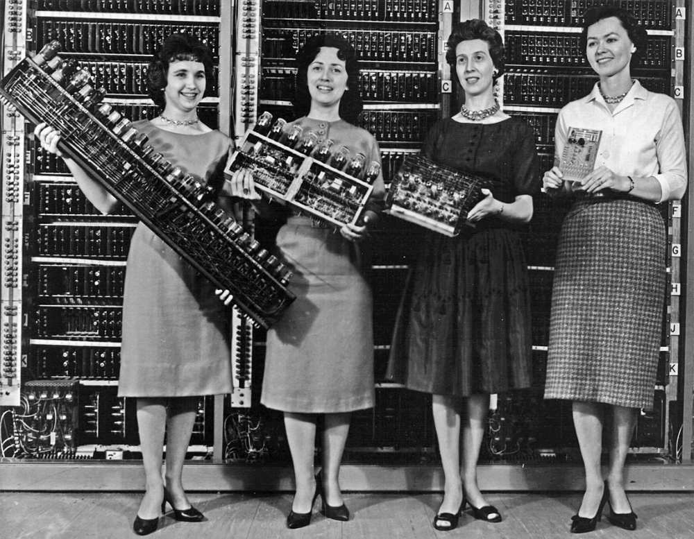
Multiple components from earlier computers from 1962. The boards and their vacuum tubes from left to right belong to: ENIAC, EDVAC, ORDVAC board, and BRLESC-I.
Scientists and engineers set out to find a replacement for the fragile and cumbersome vacuum tubes that were the source of these issues. Within this context, semiconductors gradually came to the forefront. Depending on the temperature, chemical makeup, and orientation, these materials may either be insulators or conductors.
In 1874, German scientist Karl Ferdinand Braun noticed that these crystalline solids displayed a rectifier effect. “In a large number of natural and artificial sulfur metals, […] I found that their resistance varied with the direction, intensity, and duration of the current.” When an alternating voltage was supplied, electrons could only flow through the material in one direction, producing a direct current at the opposite end.
The concept of the field effect transistor
As a result of these discoveries, engineers created the first diodes in the 1920s using lead sulfide and copper oxide. They were used in a variety of radio receivers. By adding a third electrode, a semiconductor diode can function like a vacuum tube’s triode, as first described by scientist Julius Lilienfeld in 1925. He dubbed the apparatus a field-effect transistor (FET) because of the fact that the electric field affects the semiconductor’s current flow.
Unfortunately, no practical implementations of semiconductor triodes were successful thus far. Until recently, very little was understood about the physics at play inside semiconductors. Also, the metal oxide or metal sulfide semiconductors employed back then were chemical compounds, and the wide variations in their crystalline structure and electrical characteristics during production made them unsuitable for usage. In the end, the quest for crystalline vacuum tube replacements appeared fruitless.
The first approaches for transistors
The transistor wouldn’t exist without the discovery of semiconductors like germanium and silicon. They, along with many other electronic components, owe their existence to the crystalline solids’ unique electronic characteristics. There is a good reason why the semiconductor sector has become a multibillion-dollar, internationally competitive industry.
What matters is the bandgap
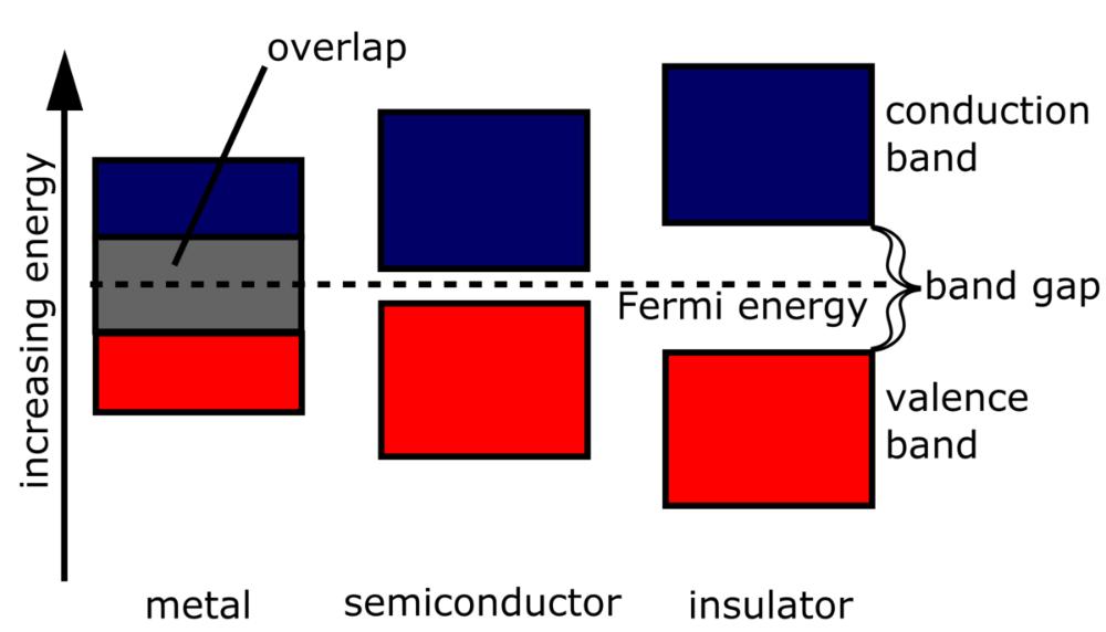
This image compares the bandgap in conductors, semiconductors, and insulators. (Credit: Energy Education)
Beginning in the late 1930s, semiconductors started their meteoric rise to prominence. Around this time, researchers had finally figured out the atomic-level causes of a semiconductor’s inconsistent electrical conductivity. They found that, unlike in metals, the electrons in these substances are restricted in their initial positions. Rather, the semiconductor electrons need to be stimulated to a particular level before they get excited and transition into the mobile state.
Semiconductors have a band gap of 0.1–4 electron volts (eV) between their insulating valence band and their mobile conduction band. When electrons in the semiconductor get energy in the form of heat, radiation, or electric current, they are able to jump the band gap. The semiconductor characteristics of substances are at their best when their atoms each contain four valence or outer electrons. Compounds like cadmium sulfide and gallium arsenide, as well as the elements silicon and germanium, fall within this category.
The effect of impurity
Also noteworthy is the discovery that germanium’s and silicon’s electrical characteristics can be tailored by the strategic introduction of foreign atoms into their crystal lattices. This doping results in either an excess of electrons (n) or a surplus of positively charged vacancies (p) in the crystal lattice, depending on the kind of impurity. Since the band gap is narrowed by the presence of these surplus local charges, the semiconductor’s local conductivity can be enhanced.
However, it was not feasible to create silicon and germanium crystals of adequate purity until after World War II, which was a necessary requirement for the fabrication of tailor-made doped semiconductors. The availability of semiconductors with a purity of 99.999 percent was only made possible by developments in crystal growth.
The attempt for the first transistor
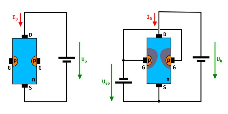
Junction field-effect transistors (JFET), and how they work. (Credit: Chtaube/CC BY SA 2.5)
As a result, several laboratories, including the illustrious Bell Laboratories in New Jersey (home to the R&D division of a major U.S. telephone corporation), began experimenting with doped germanium and silicon semiconductors. In 1945, Bell Labs’ vice president, Mervin Kelly, began a research effort to find an alternative to vacuum tubes that could be made from semiconductors. His choice of leaders for the cross-disciplinary team included physicist William Shockley and chemist Stanley Morgan.
Shockley and his colleagues began testing out various configurations of two semiconductor layers with variable doping levels as part of this effort. They employed an external electric field in the form of a third electrode, similar to what Lilienfeld had described before it, to affect the current flow between two electrodes (source and drain) inside the material. To do this, the controlling gate electrode must be situated in an n-doped area of the semiconductor, in contrast to the drain and source electrodes, which must be situated in a p-doped zone.
The current flowing between the two other electrodes is restricted and regulated by the voltage provided to the gate electrode, which creates an exclusion zone in its vicinity. The current flow between the source and drain electrodes can be modulated by varying the size of the non-conducting exclusion zone, which acts like a lock gate. These days, we refer to this basic kind of field-effect transistor by its more modern name, a junction field-effect transistor (JFET).
Two independent groups
In 1945, Shockley and his colleagues produced a germanium-based junction field-effect transistor, but the external field’s modulating effect was too weak for practical application. Therefore, Shockley tasked two members of his semiconductor research team, John Bardeen and Walter Brattain, with digging more into the matter. He, too, originally looked elsewhere for answers.
On the other side of the Atlantic, two German physicists named Heinrich Welker and Herbert Mataré were tackling the same issue and, like their American counterparts, were successful in putting the principle into practice for the first time in 1945 by experimenting with precursors to the junction field-effect transistor. Unfortunately, the expected results were still too modest, just as they had been for Shockley and his group.
The two groups were now developing more effective transistor technology apart from one another.
Toward the first transistor
It seemed like a major development was on the horizon by the autumn of 1947. John Bardeen and Walter Brattain, two semiconductor researchers working at Bell Labs in New Jersey, had identified the root cause of the early transistor experiments’ failure. Their group’s transistor models, despite some promising methods, stubbornly refused to operate, responding only very weakly to the applied control field.
The scientists found that the early versions of field-effect transistors had insufficient semiconductor penetration for the regulating electric field of the control electrode. This field regulates the flow of electricity, and its failure meant that the “lock gate” was not working as intended. Instead, the material’s electrons were trapped in a thin barrier layer just below the surface. Because of this, the candidate transistor could no longer benefit from the regulatory action.
A plastic wedge, gold foil, and germanium
Brattain and Bardeen started tinkering with a new building approach to see if they could find a workable answer. In this instance, a germanium plate was set above a metal base. This was n-doped, meaning that it had an abnormally high concentration of free electrons brought about by the incorporation of a foreign element, most often phosphorus or arsenic. Afterward, a very thin layer of p-doped germanium was grown on top. Boron and other alien atoms flooded this layer with “holes,” or a plethora of positive charges.
The aha moment finally arrived when Brattain and Bardeen came up with the idea of using a triangular plastic wedge linked to a spring and then wrapping it all in gold foil. They created two closely spaced contact points by scoring the conductive gold foil at the wedge’s tip. These were now suitable for use as two separate electrodes, with each one connecting to a separate circuit through its conductive metal base.
The first test of Brattain and Bardeen’s transistor model was performed on December 16, 1947, at their lab. It functioned, with a weak current flowing from the emitter side of the gold tip to the base and a corresponding change in the current flow in the second circuit, the latter of which was dependent on the amount of current provided to the first gold electrode.
The device worked as a variable switch and amplifier, increasing the input signal by a factor of a thousand, precisely as expected. After doing “the most important experiment” of his life, Brattain informed his team on the way home that night. But he didn’t say what it was just yet.
The first functional transistor
On December 23, 1947, the two scientists finally showed their discovery to Bell Labs’ upper management. They used a microphone and a loudspeaker to show off the transistor’s amplification capabilities during the internal demonstration. The microphone was hooked up to the little circuit of the emitter electrode, while the loudspeaker was linked to the second circuit. This meant that the speaker had to faithfully duplicate the original sound in order for the transistor to have worked.
It was at this point that Brattain and Bardeen realized their dream of creating the first operational transistor. Finally, a semiconductor-based miniaturized component to replace bulky vacuum tubes has been created. At a press conference held by Ball Laboratories on June 30, 1948, the two scientists revealed their new invention to the world.
The double-point contact transistor
The point-contact transistor is based on the basic design idea pioneered by Brattain and Bardeen. These bipolar transistors differ from the prevalent field-effect transistors in that both positive and negative charge carriers participate in the amplification process. To rephrase, the “holes” and the “electrons” in the semiconductor are both activated or mobilized.
In 1951, mass-produced point-contact transistors were used in the construction of a variety of products including telephone switchboards, hearing aids, oscillators, and even the first prototypes of television sets. These devices were the quickest switching transistors available up to 1953. In 1956, Brattain and Bardeen were honored with the Nobel Prize in Physics for their work on this.
Aside from the two American scientists, two German physicists, Herbert Mataré and Heinrich Welker, independently developed a very similar concept to the point-contact transistor without knowing about the progress being made at Bell Labs. Similarly, they built a functional point-contact transistor in 1948, although they were behind the competition.
The first bipolar transistor
In 1947, two American scientists named John Bardeen and Walter Brattain devised the first point-contact transistor, and it was a significant advancement in electronics but not yet practical as the backbone of electronics and the foundation of the first computers. As a result of their thinness, the “point-contact” electrodes tended to break easily. The essential charge carriers in this transistor only flowed across a narrow region on the semiconductor’s surface, hence the amplification it could provide was poor.
However, this all changed with the invention of the bipolar junction transistor (BJT) at Bell Labs in New Jersey only six months later. After William Shockley’s original attempts to create a field-effect transistor device in 1945 were unsuccessful, he went on to construct this new device. In the first presentation of Brattain and Bardeen’s point-contact transistor, Shockley was left out. To his dismay, he was not credited as a co-inventor on the patent for the first transistor and did not play a significant role in its creation.
The fact that he wasn’t an “inventor” dampened his enthusiasm for the team’s accomplishments. “I was frustrated that my own efforts, which had after all been going on for eight years at the time, had not resulted in any significant invention.” But that was about to change.
Shockley had been studying the physics of p-n junctions in semiconductors, the activities that take place at the interface between the two differentially doped semiconductor zones, for a few months prior to this. The scientist was trying to find a method to improve the device so that charges could be transported farther than just over its small surface. Shockley created the first working transistor on New Year’s Eve, 1947, in a hotel room in Chicago.
Stacked layers
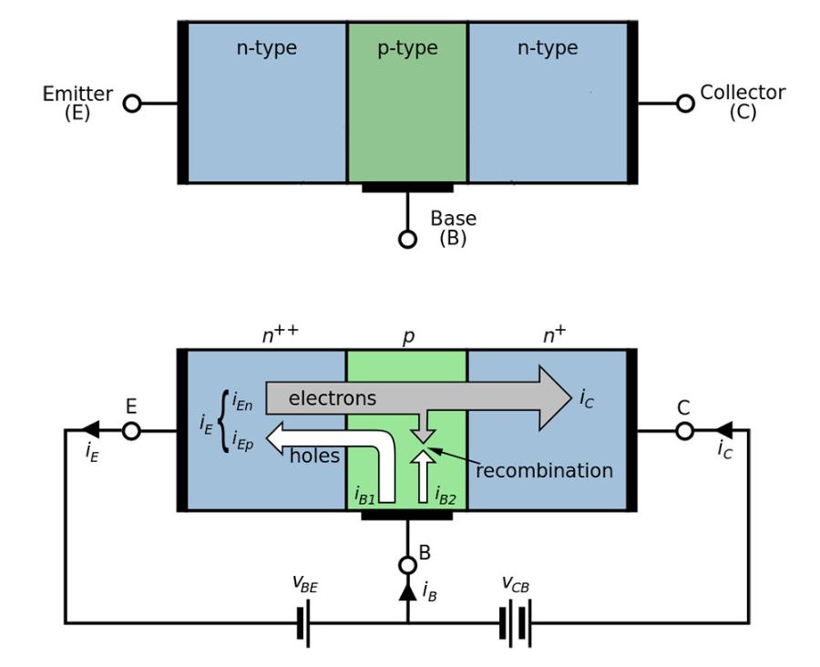
The basic operating concept of a bipolar transistor. Initially, the two n-p junctions form a barrier. Electrons flow from the emitter to the collector, and positively charged “holes” flow from the base to the emitter when a voltage is supplied to the base, reducing the barriers between the two regions.
The scientist created a sandwich out of three layers of germanium, which was the main innovation. A thin n-layer was sandwiched between two p-doped layers, or vice versa. Applying a voltage to the thin intermediate layer in such a surface transistor reduces the barriers at the n-p junctions of the semiconductor. Therefore, there is no longer any impediment to the free flow of electrons from one n-zone to the other, while positively charged holes from the p-layer can now move in the opposite direction.
Bipolar transistors were far more powerful amplifiers than point-contact transistors because they worked on a different operating principle. Plus, they were more durable. Bell Labs had filed for a patent on the transistor a few days before Shockley’s public unveiling of it at a press conference on June 30th, 1948.
Even though it wasn’t the first fully working transistor, the bipolar transistor was a major step forward for semiconductor technology and ultimately modern electronics. These reliable parts, which were simple to standardize because of advances in crystal-growing techniques, found quick adoption in applications requiring either high-speed circuits or substantial amplification. Along with John Bardeen and Walter Brattain, Shockley won the Nobel Prize in Physics in 1956 for his work on the bipolar transistor.
With their combined efforts, the three physicists sparked a wave of invention that would permanently alter the state of the art. The invention of the transistor has far-reaching consequences for our culture and economy. After all, it was because of their efforts that electronics and computer technology were able to be shrunk down to more manageable sizes.
However, a crucial step was still lacking at the dawn of the digital era.
The beginning of the silicon era
However, the shift to silicon, the semiconductor used in almost all modern electronic circuits, still remained to be achieved. It’s because most transistors in the 1950s and 1960s were fabricated from monocrystalline germanium. The lower melting temperature of this element makes it more amenable to processing, and the rapid movement of charge carriers inside the crystal lattice allows for rapid switching times.
The problem with germanium
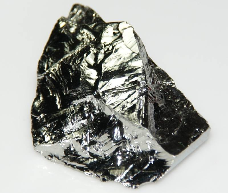
Germanium, a semiconductor, was used to create the first transistors. (Credit: Jurii, CC BY 3.0)
However, germanium does have a few drawbacks when used as a transistor material. This semiconductor’s bandgap is just 0.64 electron volts, which results in undesirable leakage currents. Once the temperature rises above around 167°F (75°C), the thermal energy is enough to make the material conductive. That’s why germanium transistors can’t be used at temperatures higher than that, since they stop switching. However, silicon is far more reliable; transistors constructed of silicon can operate at higher temperatures because of their bigger band gaps.
The difficulty in creating high-purity monocrystalline blocks of silicon stems from the material’s greater melting point of 2,580°F (1,415°C) and its increased reactivity. The electrical performance of the crystal is negatively impacted since the molten silicon reacts with practically every crucible, including quartz glass. Thus, it was initially quite difficult to manufacture silicon semiconductors with the necessary purity and doping.
Race to create the first silicon transistor
In 1954, researchers finally succeeded in overcoming these obstacles, and again, this occurred twice independently but almost simultaneously. The chemist Morris Tanenbaum at Bell Labs developed a process by which the doping rate of the silicon could be controlled while the single crystal was being pulled out of the melt. Thus, on January 26, 1954, the team developed the first n-p-n silicon transistor that had a reliable amplification performance. Bell Labs, however, initially chose not to share or patent this discovery.
Simultaneously, Gordon Teal, a chemist who had previously worked at Bell Labs, was developing a method at Texas Instruments to create silicon semiconductors with the needed characteristics. Because of this lack of purity, Teal’s team devised a method to make the interlayer of the transistor sandwich exceedingly thin, on the order of 25 micrometers. As a result, the semiconductor’s charge carriers were able to traverse this barrier, despite the presence of certain impurities. A functional n-p-n silicon transistor was developed on April 14, 1954.
Silicon has replaced germanium as the dominant semiconductor in modern transistors.
A new age
“Contrary to what my colleagues have told you about the gloomy prospects for silicon transistors: I have several of them in my pocket right now,” Teal said at a technical conference on May 10, 1954, marking an early presentation of his new silicon transistor. This was in stark contrast to Bell Labs’ decision not to announce their breakthrough.
Teal then provided a concrete example of the benefits of these components by submerging a germanium transistor attached to a loudspeaker in hot oil, at which point the music abruptly stopped. He then tried it using a silicon transistor, and the sound remained intact. The PR stunt was successful; the Teal technique was adopted, in part because the rival method was more difficult to standardize. That’s how Texas Instruments got the ball rolling on mass-producing silicon transistors.
It was this discovery that ushered in the “silicon age” and paved the way for the explosive growth of the computer and semiconductor industries. New transistor designs allowed for mass manufacture, downsizing, and integration into integrated circuits, and silicon transistors gradually displaced older germanium devices during the 1960s and 1970s.
These semiconductors made it possible to carry about and operate on computers anywhere, and they also powered global communication infrastructure. The transistor’s reputation as the “nerve cell” of the computer age is well-deserved. It’s safe to say that life as we know it now couldn’t exist without the invention of the transistor.
One of the most outstanding achievements of the human brain is its ability to learn. Neuromorphic computing attempts to transfer this fundamental brain function to machines. In this way, these computers learn in a similar way to us. But how does neuromorphic computing work? And what are the advantages of such AI systems modeled on the brain?
From the medieval Golem to the Terminator, from Metropolis to “Wall-E,” understanding the human brain, harnessing its properties, and endowing inanimate matter with human capabilities is a frequently addressed, usually threatening, often useful, but always fascinating topic. But how realistic are these ideas in today’s world? And what possibilities do we have at all to explore and imitate such a complex system as the brain?
Researchers are trying to do just that: they are working on constructing computers modeled on the brain. These neuromorphic systems also learn similarly to us at the level of their function and structure. Initial successes have already been achieved.
The brain as a model
Only at first glance does the brain appear to be a grateful research object: it is a manageable size, and as long as scientists are content with mouse brains, there is no shortage of material to study. But the true conditions for brain researchers look different.
With more than 100 billion nerve cells, the brain is the most complex organ in the human body; only in a living organism can it be observed at work. One of its most essential characteristics quickly becomes clear: the whole is more than the sum of its parts. The brain is not just a collection of tens of billions of nerve cells; it is the complex interconnections between the nerve cells that allow us to think and learn.
20,000 genes for the brain
At the beginning of development, the brain emerges from a single cell. So there must be rules that govern how the nerve cells interact during embryonic development. According to current knowledge, these rules can only be stored in our genetic material. It is assumed that about one-third of the approximately 20,000 genes in the human genome are required for brain development; this alone indicates the extraordinary complexity of the organ.
So how can we approach this extraordinary biological complexity with the goal of having machines mimic thought processes, i.e., create “artificial intelligence” (AI)?
Artificial intelligence is already producing some impressive results, such as the victories of machines over the best human chess players. However, not only traditional board games such as chess or Go, but also modern computer-based real-time strategy games can be successfully contested by machines. Researchers demonstrated this using the online game “Starcraft,” among others.
AI systems have also already mastered poker, including bluffs. AI systems can steer vehicles through heavy traffic with virtually no accidents or identify people in the live video data of thousands of surveillance cameras. These are all examples of machine learning achievements that already exist today.
Principles adopted from nature
What helped artificial intelligence achieve this breakthrough was the adoption of principles from nature. These include the concept of the multilayer nerve network, the imitation of which makes it possible to approximate even the most complicated relationships. It also includes the observation that the calculations must be closely linked to the necessary memory; otherwise, the transport of the data becomes a bottleneck.
Seen in this light, the progress of artificial intelligence is thus based primarily on the imitation of biomorphic design principles.
How does neuromorphic computing work?
When the first scientific foundations for the machine learning methods currently in use were developed in the 1950s, people had only rough ideas about how learning in the brain worked at the neuron level. The algorithms that resulted are undoubtedly very powerful, but it is equally undeniable that these procedures do not occur in nature in the way they are implemented today.
Learning with weaknesses
One could speculate that many of the limitations of artificial intelligence today are based on this shortcoming. For example, a typical weakness of AI systems is their dependence on a vast amount of learning examples; another weakness is their lack of ability to abstract or generalize correctly. This can lead, for example, to AI systems developing “biases.”
Previous AI systems require enormous amounts of data to learn.
The lack of embedding in a continuous time sequence is also a deficit in current AI systems. But only then can learning, adaptation to the environment, and action be closely interwoven, determined, and coordinated by a common internal state. Only when machines possess these capabilities will it be possible for them to independently take on complex tasks in a natural environment.
Taking a cue from reality
How can these weaknesses be addressed and solved? Scientists try to rely on “neuromorphic computing,” a research direction whose basic assumption is that one only needs to study the natural model closely enough and understand the mechanisms of nature well enough to obtain answers.
The goal of neuromorphic computing is to transfer complete knowledge about the function of the natural nervous system to artificial neural systems; such a maximally biologically inspired artificial intelligence should ideally show superior results.
However, there are also good reasons why other AI researchers rely more on conventional methods instead of incorporating the knowledge of neuroscience. One of these reasons is the complex way nerve cells communicate with each other in nature: Each individual nerve cell makes contact with about a thousand, and some even millions, of other cells. If you wanted to reproduce this natural behavior with computer systems, you would have to send at least a thousand messages for each signal from each nerve cell and distribute them to the corresponding recipient cells.
Flexible connections
To make matters worse, the natural connections between nerve cells are not statically fixed but are constantly changing. Every day, about 10 percent of all neuronal connections in our brains are broken and replaced by new ones. Many external conditions determine which connections are dissolved and which are weakened or strengthened; we only have a rudimentary understanding of these conditions.
What we currently know, however, is that the signals of complete populations of nerve cells form spatial and temporal patterns and that the targeted rewiring of connections is learned. With this in mind, then, the broader question is: How can neuromorphic computation help us understand the mechanisms of learning and the assembly, disassembly, and reassembly of neuronal connections?
Why neuromorphic computing has a future
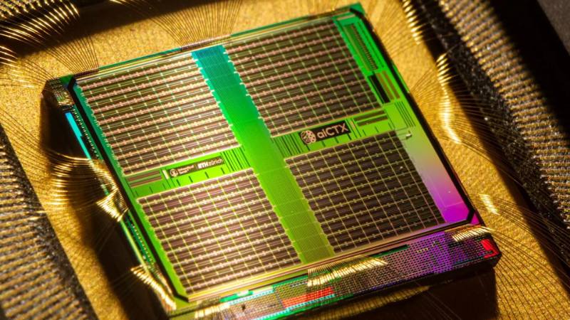
This is a neuromorphic chip. They contain hundreds of artificial nerve cells and tens of thousands of synapses. Credit: UZH, ETHZ, USZ
Some scientists simply consider neuromorphic computing to be a redundant path. With the steady increase in the power of mainframe computers, one of their arguments goes, the deficits described would disappear by themselves. The last decade, however, has shown that the expectations placed on mainframes have far exceeded what is actually technically possible.
The miniaturization of electronics, the basis of our computer technology, has slowed down considerably; in expert circles, the current discussion is no longer whether miniaturization will ever come to an end but when it will. For some time now, the energy consumption of circuits has also not been decreasing as fast as would be necessary if we wanted to match the performance increases of the past decades.
Artificial synapses on a silicon chip
Neuromorphic computing appears to be a pioneering approach to realizing biologically inspired artificial intelligence. Neuromorphic computing is about transferring the currently known biological structures of the nervous system as directly as possible to electronic circuits.
For example, scientists have succeeded in reproducing individual neurons together with their synapses—the contact points between nerve cells at which impulses are transmitted—as microelectronic circuits on silicon chips. These circuits have as many properties as possible in common with their natural counterparts; the physical model incorporates all the biological knowledge available at the current state of research. Other research teams have constructed artificial synapses based on magnetic circuits or photonic devices.
The limitations of what is currently feasible are partly imposed by neuroscience, partly by microelectronics: Microelectronics, for example, does not allow the nerve cell circuits responsible for learning to be reproduced in their full complexity, but it does make it possible not only to imitate the speed of natural processes but even to accelerate them significantly.
Computing with the hybrid plasticity model
Neuromorphic systems are at their best when it comes to learning. The findings that neuroscientists have gained in researching the brain’s ability to learn and the interconnection of neurons can be directly transferred to electronic models and tested.
A first model
The new “hybrid plasticity model” incorporates insights from neuroscience, electronics, and computer science in equal measure. For each possible connection between electronic neurons, the plasticity model holds a circuit ready to measure the signal flow. A conventional computer system could never perform this task nearly as efficiently and compactly. All signals must be monitored simultaneously, a task that nature easily masters with quadrillions of synapses firing simultaneously.
Compared to the natural model, our current electronic systems are only modest miniature versions. In the future, neuromorphic systems with up to a trillion connections will be possible. This would make it possible to test the learning of complex functions, such as the movements of humanoid robots.
The crucial factor here is that the parallel measurements of all signal flow between nerve cells must be processed by a special computer core within the same microchip. Only then can the computer core quickly and directly evaluate the measurement results for all signal flows without having to exchange information over distances of more than a few millimeters.
Fast learning even with simple rules
Because the hybrid plasticity model is a freely programmable microprocessor, scientists can determine the rules according to which the connections between the nerve cells are to be changed.
Experiments have shown that even relatively simple rules lead to stable learning results and efficient use of existing connections in a short time if they take into account the different temporal and spatial structures in the signals according to their biological models.
This learning is “hybrid” in the sense of a mixture of a physical and a virtual replica of nature. Mathematics and engineering, two fundamental cultural techniques of humans, are needed to get one step closer to understanding one of the most fundamental abilities of animate nature—the principles of learning of nervous systems. It is precisely this ability to learn that makes the phenomenon of “culture” possible in the first place.
Photons instead of electrons could shape the computer technology of the future. This is because light can be used to make circuits even smaller and computers even faster. The optical hardware alternatives open up the possibility for fascinating applications, for example in the field of artificial intelligence, and high-performance computers that come close to the way the human brain works.
Scientists, mainly experimental physicists, all over the world are researching nanophotonics and working to realize integrated optical circuits for artificial intelligence and optical quantum computing.
How exposure shapes semiconductor structures
In photography, the effects of hard and soft light are well known. Hard light can be used to illuminate the surroundings with clearly defined, sharp contours in the cast shadow. Soft light makes the image more diffuse and blurs outlines. The decisive factor for the respective effect is the size of the light source in comparison to the illuminated object: a relatively small light source leads to hard shadows, and an extended light source leads to softer, blurred contours.
Down to the nanoscale
Hybrid nanowires with polarization of light. (Credit: June Sang Lee, University of Oxford)
Playing with sharpness and blur does not only allow visual art impressive design possibilities. Sharp contours are also desirable when it comes to creating defined structures for semiconductor technology on very small length scales. However, diffraction of light at very small structures causes clear patterns to soften, which always happens when the scales are in the range of the optical wavelength and thus on the nanoscale.
These diffraction effects dictate the minimum resolution that can be achieved when exposed to a given wavelength or color of light. To achieve very fine nanostructures or very densely packed patterns, really hard light would be ideal. Especially since light affects not only the contours but also the properties of the exposed materials, such as in photolithography, an important method for manufacturing semiconductor devices.
The importance of coating
To create nanopatterns, photoresists are used in semiconductor technology. The solubility of photoresists depends on how they are exposed: There are resists that cure or chemically crosslink upon exposure, and there are resists that soften when exposed to the light of a certain wavelength. Curing coatings are suitable for protecting materials, while softening coatings are used, for example, to define areas where further processing steps are to take place.
The sophisticated sequence of exposures with both types of photoresists is the basis for producing nanostructures that process electrical or optical signals and can be used as integrated building blocks (chips) for electronics and optics. For so-called integrated optics, i.e., optics on a chip basis, scientists usually aim for nanostructures that are smaller than one micrometer. For comparison, hair has a diameter of about 50 micrometers.
Light can be introduced into very small nanostructures with the help of so-called waveguides. This makes circuits possible in which light particles, called photons, act instead of electrons.
Advantage of photonic computers: Light instead of electrons
Since photons move at the speed of light in a vacuum, they always beat out electrons, which are much heavier particles.
Photonic circuits are interesting for all applications that require data to be processed very quickly and without consuming large amounts of energy. This is because light particles work in them instead of electrons. This opens the door to completely new optical computer architectures that do not work like traditional electronic computers but are modeled on the way the human brain works.
Modeled on the brain
The focus is on the development and improvement of these computing architectures. Neuromorphic computers inspired by the construction and operation of the human brain are important for providing hardware for artificial intelligence (AI). AI applications have already arrived in many areas of our everyday lives. For example, they help with speech recognition, encrypt data on smartphones, support search functions, are used for pattern recognition on the Internet, and are essential for safety in autonomous driving.
All these applications pose enormous challenges for conventional electronic computers, because data storage and processing are carried out separately in them. This type of electronic architecture makes it necessary to exchange data continuously via special systems known as bus systems, which leads to sequential clocking and limits data throughput.
Analog computing
The human brain handles data completely differently: They are processed locally with very high parallelism, and processing is often analog, i.e., continuous, rather than digital, i.e., in steps. This is important for all computational operations required in AI. “Photonic neuromorphic computing” promises to meet these high demands.
Photonic neuromorphic computers use light to perform addition and multiplication as elementary mathematical computational operations. The actual computational task is translated into the encoding of the numbers to be computed together as well as the measurement of the result. Photonic neuromorphic computers can do this in a single step because light particles, unlike electrons, have many degrees of freedom that allow for inherent, simultaneous data processing—this is the special charm of optical computing methods.
How photonic chips calculate
Our brains – and also artificial neural networks – process information using multi-layered networks of parallel nodes. (Image: ScienceDirect)
In electronic systems, it is necessary to perform many individual operations one after the other. For data transmission using optical fibers, for example, the wavelength of light is exploited so that data can be exchanged in many colors simultaneously over the same optical fiber.
Faster through parallel processing
This principle can also be used for photonic computers: Different computing operations are encoded on different colors and performed in parallel in the same optical computing system. Parallel processing offers enormous speed increases due to increased clock frequency; the calculations are performed at the speed of light, as it were. Photonic computers can not only compute much faster than electronic systems, but they can also scale in a dimension that is fundamentally unavailable to traditional computers.
Thanks to advances in materials science and integrated optics, photonic circuits can now be designed and simulated on the computer and then manufactured in factories. Fortunately, silicon can be used as a waveguide material, which is also highly compatible with the methods used in the semiconductor industry.
With matrices and vectors
The provision of all these capacities makes it possible to combine individual components into large-scale systems. For optical computing, this means: Small circuits are interconnected to form powerful arithmetic units that perform many multiplications and additions in parallel. This is done with the aid of arithmetic grids or matrices. The inputs of the numbers to be multiplied are available in parallel as vectors.
Based on these, the photonic chips perform matrix-vector calculations using light, with very high data throughput and very low energy consumption. Synthetic structures that mimic nerve cell networks are already being used today in artificial intelligence for cognitive processes. Matrix-vector multiplications are central computations in these neural networks. However, they have to be performed repeatedly, which takes a lot of time and energy.
To save time and energy, scientists try to have the central computational steps performed by special accelerator systems that are optimized for this kind of computational operation and can make them efficiently available for further computations. This is where photonic hardware accelerators come into play: they allow very fast data processing and provide a very large computing capacity in the long term.
Hybrid computing with electrons and light
Photonic computers are very well suited for special operations, while other operations can be better mapped in electronic hardware. The ideal would be “hybrid computers” that work electronically and at the same time contain photonic accelerators. So far, it is still difficult to integrate photonic accelerators into existing electronic computing systems. However, these approaches are attractive models for future high-performance computers that physicists are exploring to satisfy the computational appetite of new AI applications, even in the long term.
Where photonic modules have an advantage
The very high processing speeds make photonic computing modules interesting, for example, for object recognition in autonomous driving, an essential safety requirement. For this purpose, camera and sensor systems record the environment, and the computer must interpret the data so that it can react dynamically to what is happening on the road. AI processes, especially neural networks, are a central component of this.
How fast the overall system reacts is determined by the computing time of the system components: The faster the object detection, the faster the vehicle can be corrected; the accelerator systems thus directly influence the safety of the overall system.
Other interesting applications include training neural networks, which is very time and energy-consuming. Photonic matrix-vector multipliers can be used for this purpose. They offer the advantage of high data throughput, they can be efficiently adapted to different requirements, and they contribute significantly to a reduction in energy consumption.
Phase change as a chip designer
Photonic computers can also be reprogrammed in a variety of ways. One elegant solution is via phase-change materials, such as those used on rewritable DVDs. If these materials exist as hard crystals, they are metal-like. If the crystal structure is disordered or amorphous, the materials are glass-like and transparent. Both states can be very accurately adjusted by exposure to short laser pulses.
The change in material state is used as a basic principle for optical data storage on DVDs, for which the multiplicands of the material property are encoded: Metal-like, hard crystal states represent a logical zero, and glass-like, soft crystal states represent a logical one. Once set, the states are maintained over very long periods of time, up to decades, without the need for external energy input.
Last but not least, it is attractive for practical applications that even very small structures of a phase change material have very large effects on the light via the waveguide used. This allows scientists to reduce the size of the devices and effectively use the space on a chip.
The softness and hardness of light outline a fascinating field of tension: on the one hand, the precise formation of structures with the help of the properties of light, and on the other hand, the adjustment of the degree of hardness of materials through light modifications. Skillful exploitation of this interplay makes it possible to design new lithography processes and new optical methods for data processing.
The transition regions between the two extremes are particularly exciting, such as mixed states of phase change materials that contain both ordered crystalline and disordered components. Equipped with this toolbox, it is then certainly possible to solve even the hardest problems of computer architecture design.
Long before the discovery of the modern computer, Charles Babbage designed machines that could handle complex mathematical operations and developed the world’s first programmable computing device. As a brilliant mathematician, Babbage contributed to various fields such as the development of railways, and business productivity. There is general consensus that the English philosopher and inventor Charles Babbage should be recognized as the “father of the computer.” The “Analytical Engine,” his design for a mechanical computer, is his claim to fame. The Analytical Engine was created by Babbage with the intention of automating mathematical operations through the use of punch cards. Although Babbage was unable to build a fully functional model of his Analytical Engine, his theories helped pave the way for the creation of today’s computers. In mathematics, he is credited for creating the idea of algebraic invariants and the notion of a “difference engine,” a mechanical device that could automatically calculate mathematical tables.
Who was Charles Babbage?
Babbage was quite curious in his childhood. In his autobiography, he says he made it customary that whenever he received a new toy, he asked his mother, “What’s in it?” Another custom was to disassemble them to understand how they worked. This sense of curiosity made led Babbage to understand machines and their mechanisms at a very young age.
In 1810, he began studying mathematics at Trinity College, Cambridge University. At that time, mathematicians and engineers were making calculations by consulting books filled with charts. These books included trigonometric functions (sinus, cosine, and tangent) and logarithmic charts. There were hundreds of tables and thousands of numbers on each table. The values in the charts were extracted by hand.
In 1812, Charles Babbage moved to Peterhouse College. During his studies in the school’s library, he discovered numerous errors in the numerical charts. These appeared to be human errors. Various mechanical calculators were used at the time. However, these tools were only useful for a few tasks. Based on his observations, Babbage designed a machine that could calculate these charts quickly and eliminate human error.
In 1822, he submitted a proposal to the Royal Astronomical Society for a calculator. Babbage also commissioned an engineer to supervise the work. The engineer began working in a workshop near Babbage’s house, where there was a machine tool carefully designed by Babbage. To carry out this gigantic task, Babbage was constantly seeking and receiving financial assistance from the British government.
The Difference Engine of Charles Babbage
The working replica of the Difference Engine designed by Charles Babbage.
Charles Babbage called the device he proposed the “Difference Engine.” Perhaps because of the complexity of the work, some disputes arose between Babbage and the engineer, and the machine was never finished. In 1842, the government ceased financial support. Babbage later improved the machine and named it “Difference Engine 2.” In 1991, the London Science Museum recreated Babbage’s design and made the machine operate. In 2005, a printer was added to Babbage’s design. Both devices worked perfectly.
When his father, wife, and son died in 1827, Babbage took a break from his studies and set off for a journey in Europe. During his journey, he considered a more comprehensive computing device that could carry out a series of instructions. Babbage had a machine in his head that took input through punch cards, stored answers, and also printed output with a printer. In 1835, he produced the first of many designs for an “Analytical Engine.” This machine was the pioneer of today’s programmable computers. The design consisted of 500 large technical drawings, 1,000 pages of engineering calculations, and thousands of pages of drafts. Unfortunately, this machine was never completed.
Babbage’s designs inspired the pioneers of modern computers, and he had significant influence in other fields as well. While traveling in Europe in the 1820s, Babbage toured several factories and examined the forms of production there. In 1832, he published his book “On the Economy of Machinery and Manufactures.” This work is considered the first example of productivity research in a business field and industry, now known as operations research. Babbage also applied his methods to the postal system in England. The result was the world’s first inexpensive and efficient mail system.
Later, Babbage made a Table of the Logarithms of the Natural Numbers: From 1 to 108,000 which was so well received that it was translated into so many European languages.
Babbage also studied the efficiency of the rail systems, which at that time was still fairly new. In addition to this work, he developed a special vehicle with instruments to record the shakes during a train journey and a device known as the cowcatcher for removing objects from the rails in front of the moving train.
Charles Babbage and the Analytical Engine
A working Analytical Engine designed by Charles Babbage.
Babbage’s Analytical Engine was the first known general-purpose, mechanical computer design in history. Although never finished, the concepts in the design of the machine were still in use even 100 years later. The program and data were entered via punch cards. The output consisted of a printer, a curve plotter, and a bell. The machine’s memory was capable of storing 1,000 numbers, each with 50 digits. The language of the program was very similar to the language used on the first computers that would appear 100 years later.
Loops and conditional branching were employed by the machine. There, Alan Turing‘s famous concept was actually developed much earlier than it first appeared. Although Babbage’s immediate impact on the subsequent development of calculators is debatable, engineer Howard H. Aiken, who was primarily responsible for IBM’s 1944 Harvard Mark 1 (the first large-scale, automated digital computer in the United States), said of Babbage’s writings on the Analytical Engine: “There’s my education in computers, right there; this is the whole thing, everything I took out of a book.” That is why Charles Babbage is the father of computer.
The death of Charles Babbage
In 1811, Babbage succeeded Isaac Newton, Isaac Barrow, Bishop Turton, and Professor Airey as Lucasian professor of mathematics. He belonged to several academic and literary organizations and was a Fellow of the Royal Society.
In London, England, Babbage passed away on October 18, 1871, at the age of 79. The autopsy results indicated that Charles Babbage died of kidney failure, most likely due to a severe urinary tract infection. Babbage is known as one of the forefathers of the modern computer due to his influential work in computer science and his novel approach to mechanical engineering.
Charles Babbage quotes
“Errors using inadequate data are much less than those using no data at all.”
“The economy of human time is the next advantage of machinery in manufactures.”
“On two occasions I have been asked, ‘Pray, Mr. Babbage, if you put into the machine wrong figures, will the right answers come out?’ I am not able rightly to apprehend the kind of confusion of ideas that could provoke such a question.”
“As soon as an Analytical Engine exists, it will necessarily guide the future course of science.”
“At each increase of knowledge, as well as on the contrivance of every new tool, human labour becomes abridged.”
“What is there in a name? It is merely an empty basket, until you put something into it.”
“I wish to God these calculations had been executed by steam.”
“I have no desire to write my own biography, as long as I have strength and means to do better work.”
Bibliography
The background image in the cover picture: Baranozdemir/Getty Images
Ole Immanuel Franksen, Mr. Babbage’s Secret. The Tale of a Cypher – and APL (Birkerød, Denmark: Strandbergs Forlag, 1984.
What were Alan Turing’s major contributions to the field of mathematics?
Alan Turing made significant contributions to the field of mathematics, including his invention of the Universal Turing Machine, a theoretical device that is widely considered to be the precursor to modern computers. He also made important contributions to the fields of logic, computability theory, and artificial intelligence, among others.
How did Alan Turing’s work during World War II impact the outcome of the war?
Alan Turing’s work in breaking the German Enigma code during World War II played a crucial role in Allied victory. His decryption of encrypted messages allowed the Allies to anticipate and disrupt German military movements, ultimately leading to the defeat of Germany.
What was Alan Turing’s role in the development of early computers?
Alan Turing is often considered to be one of the founding fathers of modern computing. His invention of the Universal Turing Machine laid the groundwork for the development of digital computers, and his work on algorithms and machine intelligence helped to shape the field of computer science.
What challenges did Alan Turing face during his lifetime?
Alan Turing faced numerous challenges during his lifetime, including discrimination for his homosexuality, which was illegal in England at the time. He was convicted of homosexuality in 1952 and forced to undergo chemical castration. He died two years later, and it is widely believed that his death by suicide was a result of the treatment he received.
What is the significance of the Turing Test in the field of artificial intelligence?
The Turing Test, which was proposed by Alan Turing in 1950, is a test of a machine’s ability to exhibit intelligent behavior that is indistinguishable from that of a human. The test has been widely used in the field of artificial intelligence as a benchmark for evaluating the intelligence of machines. The Turing Test has played a significant role in shaping the development of artificial intelligence, and it remains an important topic of research and debate in the field today.
Alan Turing deserves to be called the father of modern computer science. In the years before World War II, he built the theoretical infrastructure for multipurpose machines that formed models for the computer in its most general shape. His seminal 1936 essay, “On Computable Numbers, with an Application to the Entscheidungsproblem,” was later realized as the way he foretold what modern computers can do. During the war, he helped to develop computing devices that were said to shorten the war by two years by deciphering encrypted enemy messages that were thought to be indecipherable. Unlike some theorists, he was also willing to work on practical issues. Thus, he was happy to use a soldering iron in the same way he was grappling with a math problem: by approaching it from a unique angle.
Who was Alan Turing?
Alan Mathison Turing was born on June 23, 1912. His father was a civil servant in India. His parents returned to Maida Vale, London, England, before his birth. At the age of 14, he was sent to Sherborne School, the traditional public school in Dorset, South England. Alan’s interest in science was noticed by the teachers at the school, but he did not find any support in this conservative institution. For example, before learning calculus, he was able to solve advanced mathematical problems developed with the first principles. At the age of 16, he came across Albert Einstein‘s work and understood it. While at school, he became intimate with a student, but his friend died during their last term at Sherborne. This event had a traumatic effect on Alan, and he lost all religious beliefs quickly. Over time, he became an atheist.
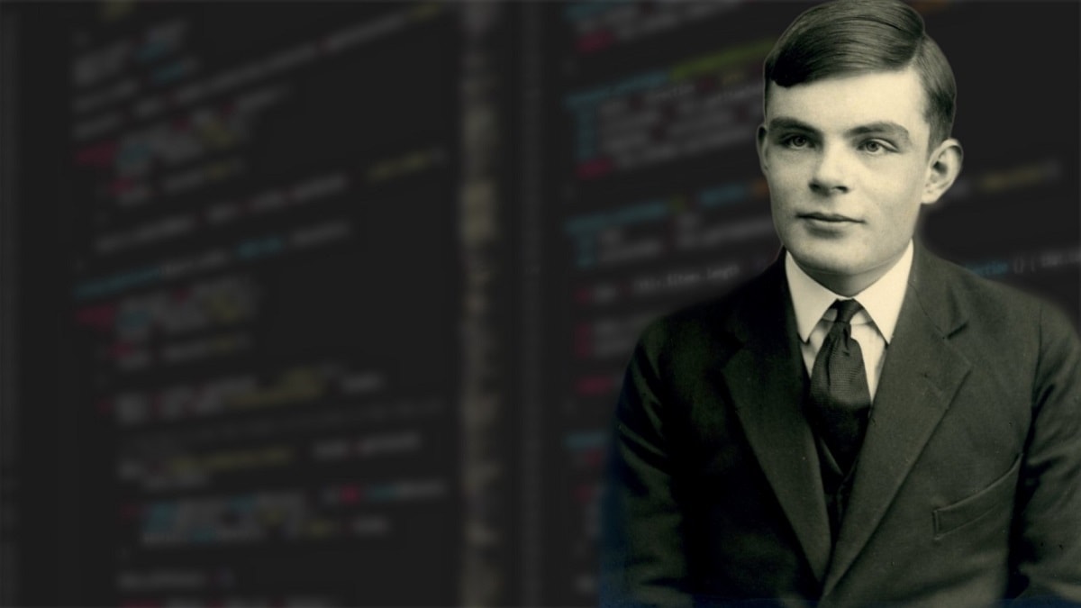
Alan Turing.
Alan Turing continued his education by attending King’s College, Cambridge, from 1931 to 1934, where he graduated with honors. He was later chosen as an academic member of the college. In 1936, he delivered his groundbreaking article on computable numbers that would form the basis of his career. This article describes the concept of a machine that can perform calculations, especially a universal machine that can calculate a wide variety of mathematical problems. Turing’s idea of universality has transformed into the concept of “programmability in computers” today. In a 1939 article, in the context of the human-computer, he stated, “A man provided with paper, pencil, and eraser and subject to strict discipline is in effect a universal machine.“
Turing’s efforts enhanced German mathematician Kurt Gödel’s research in 1931 and led to the use of the term “Turing machine” for this universal machine. Alan Turing showed that this type of machine can perform any mathematical calculation that can be expressed with an algorithm. The Entscheidungsproblem, which he mentions in his 1936 article, was the mathematical problem of whether there is always an algorithm that could judge the correctness or falsity of a mathematical proposition, put forward by German mathematician David Hilbert in 1928.
Church-Turing thesis
The three-wheel Enigma cipher that the Germans thought produced an unsolvable cipher and therefore used for their military plans.
Alan Turing also demonstrated the unsolvability of the problem by showing the impossibility of algorithmically determining the capabilities of any particular Turing machine. This notion, known today as the stopping problem, is a troubling issue for mathematicians. The Turing machine has remained an important concept in computability theory to this day. Although an abstract concept (Turing did not originally think of making such a machine), it could actually be done, which predicted many aspects of contemporary computer features and processes, such as input, output, memory, and programming. Alan Turing completed his doctorate in a remarkably short period, working from 1936 to 1938 at Princeton University under the supervision of American mathematician Alonzo Crunch.
They had previously developed the Church-Turing thesis, which described the nature of computability apart from Alan’s thesis, arguing that any effectively computable function produced by any means can also be calculated using the Turing machine. Although the thesis cannot be proven, it is generally accepted by mathematicians and theoretical computer scientists. Turing returned to Cambridge and attended the philosopher Ludwig Wittgenstein’s lectures on the fundamentals of mathematics. Wittgenstein said that math didn’t find the truth; it made it up, but Turing didn’t agree with this.
Decryption
Hut 6 machine room in Bletchley Park. This is where the British were trying to decrypt the enigma codes of the German army and air force.
The war brought a radical but accidental change in the direction of Turing’s career. His unique talent in math was spotted while at Cambridge, and he was invited to join Bletchley Park, the secret center of England’s efforts to crack German codes. He first started working part-time at the Government Code and Cypher School (now Government Communication Headquarters, GCHO) and then switched to working full-time.
The manual decryption process was both difficult and lengthy for a country facing an approaching enemy. Alan Turing realized that, when combined with a human’s unlimited creativity, machines could solve problems much faster and more reliably. Before the war, he had already helped try to figure out how the Germans encrypted their messages with the Enigma machine.
A few weeks after joining, he set up a machine that could help decrypt Enigma. His solution was named bombe after the earlier Polish device called bomba. Bombe (called crypt) was taking a possible simple piece of the original text and passing it through the combinations of rotors and plugboards in the Enigma. The most likely arrangements produced contradictions, thus eliminating them and leaving only a few combinations for further investigation. The machine performed a mathematical proof mechanically much more effectively than a human, or even a team, could.
What Kind of a Character was Alan Turing?
Front view of one of Turing’s original bombe machines; The bombe machines were the electromechanical tools Turing designed to decode the Enigma in Bletchley Park in 1939.
Alan Turing chose to work on the decoding of Enigma messages used in the Navy, and the reason for this was that “Nobody else was doing anything about it; it could be my job.” This was very typical for Alan, although he was comfortable cooperating with others. He developed new methods of decryption during his time at Bletchley Park. He often referred to them by slang names. One of them was the “Turingery” or “Turingismus,” which he developed in 1942. It was a manual calculation technique to find the string in the rotors of the Lorenz cipher machine, which the Germans used to encrypt high-level strategic orders. The British also deciphered this machine. The method was especially helpful because the information it gave was still true after a certain amount of time.
Alan Turing’s colleagues at Bletchley Park were aware of his unusual manners. He had chained the coffee mug to the radiator so that it would not be lost or stolen. When he came to work by bicycle, he wore a gas mask to protect him from hay fever, not fear of gas. However, with the help of his contribution to the work in Bletchley Park, he developed the world’s first programmable digital electronic computer, called Colossus. Alan Turing was awarded the OBE, the Order of Chivalry, in 1945 for his efforts during the war, but his contributions remained anonymous for years.
Tough Times for Alan
Pilot ACE’s (Automatic Computing Engine) circuits were among the first computers to store instructions, first operated in 1950 at the National Physical Laboratory, NPL.
After the war, Turing took a post at the National Physical Laboratory in Teddington, West London. Here he worked on one of the first computers, the Automatic Computing Engine, or ACE. Sadly, a simplified version of the Pilot ACE was never completed due to delays and Turing’s return to Cambridge on paid leave for a year.
He joined the University of Manchester in 1948 to study mathematics and was appointed deputy director of the university’s computer laboratory. He worked on the software of the Manchester Mark 1. Alan Turing continued to think about more theoretical and abstract ideas, one of which was artificial intelligence, investigating whether a machine could think. For the possible demonstration of the machine’s intelligence, he prepared the Turing test: for a computer to pass the test, it had to be indistinguishable from real humans when in contact with a human. Despite its presumed feasibility, this test has not yet been passed and has not lost its importance today. In fact, many variants of the test are currently in use.
Alan Turing lived at a time when homosexuality was illegal in England. He was charged in 1952 for obscene behavior and lost his security clearance. He had given him two options: incarceration or taking female hormones for a year in the hopes of “curing.” From this point on, he studied morphogenesis in interdisciplinary mathematical biology, becoming particularly interested in the process that allows organisms to produce their forms. Most of these works were published until 1992, when his articles were compiled.
How Did Alan Turing Die?
Turing was found dead in his home by his maid on June 8, 1954. The cause of death was cyanide poisoning, thought to have been caused by the half-eaten apple sitting beside his bed, but the apple was never tested. It was determined that he committed suicide, but the death was likely to be an accident.
Turing was admitted to the Royal Society in 1951, a year before he fell into disfavor. He was only truly appreciated after his death. Now there are two statues erected—one in Manchester and one in Bletchley Park. There are plaques at his birthplace in London and the house where he died in Wilmslow. The British government officially apologized for the official treatment that led Alan Turing to his death in 2009. But perhaps the most appropriate is the A.M. Turing Award, which is the equivalent of the Nobel Prize awarded each year to a leading computer scientist. Even though Turing died too young at age 41, his ideas will still be used in the field of computers in the near future.
John Von Neumann: The Scientific Genius Who Pioneered the Modern Computer, Game Theory, Nuclear Deterrence, and Much More, Norman MacRae, 1999, American Mathematical Society, Chapter 8.
Hodges, Andrew (2012). Alan Turing: The Enigma. Princeton University Press. p. 87. ISBN 978-0-691-15564-7.